In the following I hope to demystify some of the aspects of neurofeedback training with bipolar placements, or at least provide substantiation for some of the statements I have been making about it. We are concerned with reward-based training with narrow-band filters that select a particular training frequency. The bipolar montage feeds a differential amplifier that senses the difference in voltage waveforms appearing at the two sites. The signal that is common to the two sites cancels out in the amplifier circuit. This helps us with respect to cancellation of electronic interference that is common to both electrodes, but the same considerations apply to the signal itself. We only get to see the differential signal between the two sites.

For reasons that will ultimately become clear, I am particularly interested in the phase dependence of the signal, mostly because this has been missing from the discussion to date. How can we best illustrate this? One would like to have the same waveform, for example a sinusoidal waveform at the center frequency of the filter, appearing at both electrodes, and to see what happens as we shift the phase between the two signals. The resulting signal would be time-dependent, which cannot be easily shown in a static graphic in a newsletter. So we will do the next-best thing: We will simulate two slightly different frequencies at the two sites. They will therefore progressively move out of phase and then back into phase in yet another sinusoidal pattern, namely at the beat frequency or the difference frequency. This can be shown as a frozen image, as we have done in Figure 1.

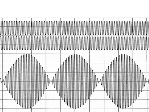
What we get is the relationship of net amplitude on relative phase shown in Figure 2. This Figure can equally well be obtained through the explicit calculation of the vector sum of the two signals. And that was in fact done to set the stage for what is to follow. The only simplifying assumption that has been made is that both signals are of the same magnitude. Note how the shape of Figure 2 is reflected in the beat frequency amplitude in Figure 1.

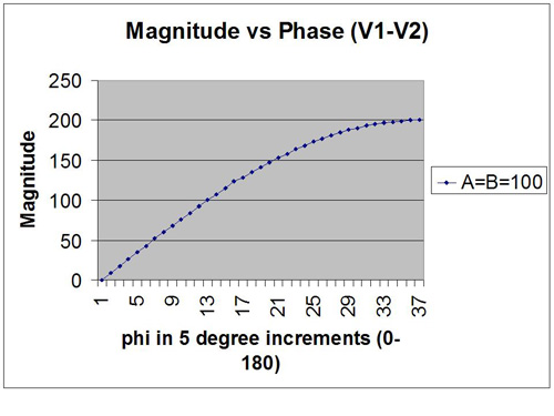
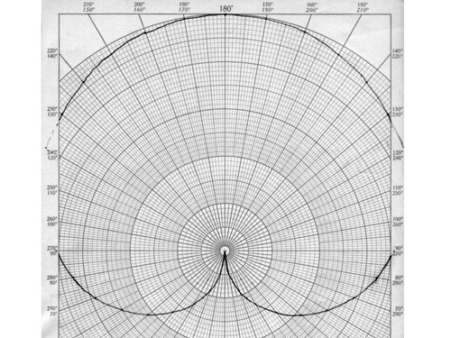
Now, given the fact that we are really dealing with vector sums and phase relationships, it lies close to hand to actually plot this equation on a polar plot. This is shown in Figure 3. In this Figure, the phase of one signal is arbitrarily set at zero degrees, and the phase of the other (i.e., the relative phase) covers the range of zero to 360 degrees. This plot is more intuitive than Figure 2, but both are identical in their content. In Figure 3 we see directly that when the two signals line up at zero degrees there is complete cancellation of the net signal. When the two signals are out of phase, on the other hand, they contribute additively. Observe that the strongest phase dependence is found near zero degree phase difference, and the weakest phase dependence is to be found near 180 degrees.

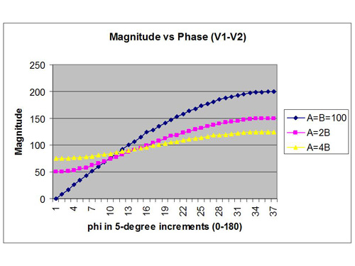
Now EEG amplitudes are not usually matched in nature, so in Figure 4 we have shown what happens for a couple of other assumptions in amplitude ratio. The phase dependence is now much softer than when the amplitudes are matched, but the phase dependence is still obvious. The implication is that phase matters, and that it does not suffice just to talk in terms of relative amplitude. But I have to grant that Figure 4 is hardly representative of what happens in the real EEG.

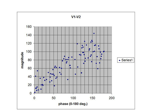
In order to simulate what might happen in an actual situation with bipolar placement, we must randomize both of the amplitudes and the phase. This is done in what is called a Monte Carlo calculation. We simply insert random values of amplitudes and phase into the vector sum equation, and see what we get for a net signal. The results are shown in Figure 5, and they are fascinating. Even when we give full range to the amplitude variables, the phase dependence of the net signal remains quite obvious. The larger net signals occur at the larger phase angles.

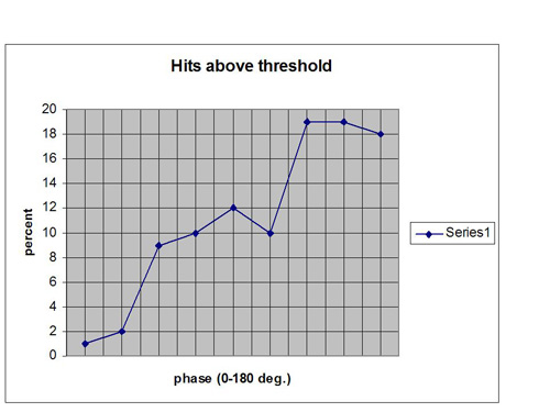
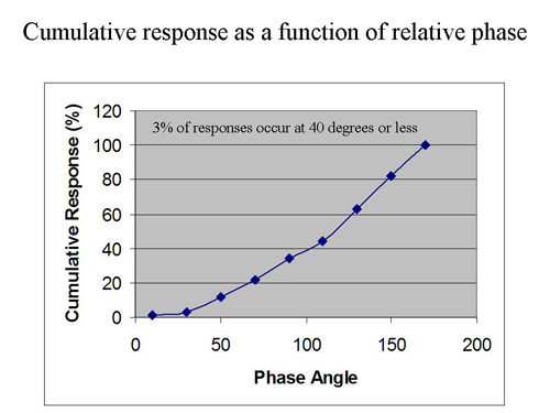
Now let us carry the simulation even further by putting our fake EEG data into a feedback configuration and applying a threshold to the net signal. We typically set our reward thresholds to yield at least 70% success. If we use that criterion with these data we will have to place our threshold at 41. The distribution of data points above that threshold are shown in Figure 6. Even more illustrative is the cumulative distribution of all hits up to a given value of phase. This is shown in Figure 7. It reveals that under the above assumptions, only about 3% of rewards are issued for phase angles less than 40 degrees. We obtain a “phase hole” around zero relative phase, a soft exclusion zone for rewards.

Thus the net signal is likely to be graced with a reward only if there is amplitude disparity between the channels, or a phase disparity, or much more likely a combination of both. The mathematics does not in fact allow us to make the argument any stronger with respect to amplitude than with respect to phase. And of course the bipolar signal does not give us any insight into the components of the signal that we have modeled up to now. All we ever get to see is the net signal.

To go beyond the simulation above we would have to introduce realism into the assumptions on the basis of some of the things we know about the EEG. For example, the EEG is much closer to a Gaussian amplitude distribution than a flat distribution. This would yield amplitude data that are slightly more correlated than we have assumed. A greater correlation in amplitude makes for a stronger phase dependence, as shown in Figure 4. This just places more of the burden of disparity on the phase variable. By the same token, if the amplitudes at the two sites are highly correlated because the electrodes are placed close together, or for reasons of pathology, the net signal will predominantly reflect relative phase.

The point of this exercise is to lay the basis for a more “agnostic” or “non-prescriptive” model of neurofeedback in which the reinforcement is not so much targeting a specific objective (such as elevating SMR amplitudes, for example) but rather a more general objective of enhancing the disparity between sites in the moment. And even this goal is nothing more than the immediate operational objective within the confines of the training rather than any kind of ultimate objective of the training. Greater disparity between sites may indeed have functional utility for the majority of clinical cases, but we don’t know that to be true and we don’t have to assume it to be true in order for the exercise to be useful. The bulk of observed EEG amplitude anomalies lie in the direction of excess amplitudes, which can be modeled in terms of excess local synchrony. To that majority of cases, a training strategy with a bias toward desynchronization may well be appropriate. But our clinical impression is that the bipolar training strategy does not just apply to such cases.

Our intent here is to be descriptive, not prescriptive. Bipolar training has been found to be quite useful clinically, and yet we have not had a satisfactory description of what actually goes on–in detail and in the moment. In particular, models based on amplitude training have foundered on the inconvenient finding that a systematic EEG change in the direction of the protocol is not observed at the training sites. So perhaps nothing is going on beyond a “subtle disturbance of the state of the system, which in turn provokes a reaction by the brain to restore proper regulation.” We call this the challenge model. Such subtle disturbances should be measurable within the session, but may not long survive the session, as Juri Kropotov has shown with respect to amplitude data, and as Richard Soutar has verified as well with coherence measurements. The above argument simply brings the variable of phase into the discussion on equal terms.

Acknowledgements: I thank John Putman for the relevant calculations.

This entry was posted on Wednesday, June 14th, 2006 at 7:35 pm and is filed under Protocols, Scientific. You can follow any responses to this entry through the RSS 2.0 feed. You can leave a response, or trackback from your own site.