by Siegfried Othmer, PhD
 I n the previous newsletter it was established that the outliers in the distribution of reaction times could not be interpreted as the tail of the Gaussian distribution. They had to be treated as a distinct phenomenon. When it came to characterizing the distribution function that characterizes the outliers, the analysis suffered from insufficient data. After all, reaction time outliers are relatively rare, so even a database of over 1500 did not give us enough to work with.
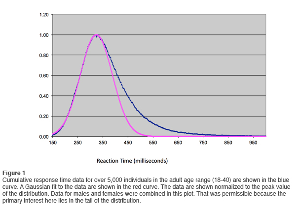
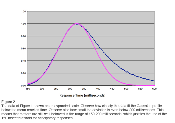
In January of 2012 we ran the analysis again, and on this occasion the database available to us exceeded 5,000. The results of the cumulative reaction time distribution are shown in Figure 1. On the vertical scale the data are normalized to the peak value. A Gaussian fit to the data is also shown. It is even more revealing to plot the data on an expanded scale, as shown in Figure 2. Observe just how well the data are represented by the Gaussian curve at reaction times at or below the mean. Small deviations are observed only below 200msec. This justifies the change we made in the QIKtest of setting the threshold of anticipatory responses at 150msec rather than the 200msec that is standard in the T.O.V.A.®.
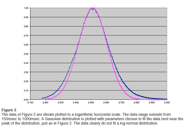
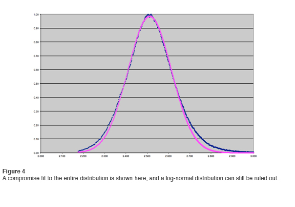
In the first newsletter we went through the exercise of fitting a log-normal distribution to the data. This is most easily done by means of logarithmic compression on the horizontal axis and fitting a Gaussian. Bear with us as we go through this exercise again with the larger data set. The results are shown in Figure 3. That the data in the tail do not fit the log-normal distribution is even more apparent than before. If the data were less clean, one would fit the curve as best one could and move on. Such a compromise fit is shown in Figure 4, but with such clean data the fit is unambiguously ruled out.
The point of this exercise is to illustrate just how tempting it is to fit a log-normal distribution to skewed data. The Gaussian distribution is so convenient to deal with that one may be inclined to overlook small deviations just for the privilege. Where might that be most relevant to people in our field? It is in the analysis of quantitative EEG data! It is well-known that the EEG band amplitudes are not Gaussian-distributed. But typically a Gaussian is fitted anyway, and nearly everyone accepts the approximation for purposes of practicality. The use of short data acquisition times assures that the data are always sufficiently noisy, so that the inconvenient tail resides in a state of ambiguity and can therefore be swept under the rug. Good science may well have gone down the drain over the years. It is likely that once one is forced out of the comfort zone of the Gaussian assumption, different models will appeal. That was certainly the case here for the reaction time distribution. The most revealing information lay in the extreme tail of the distribution.
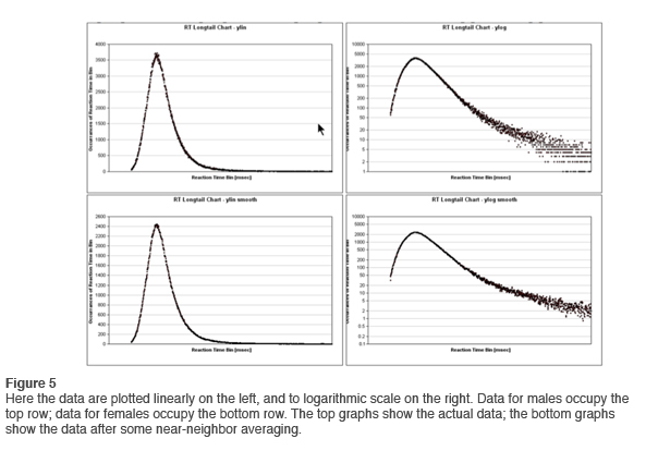
In newsletter #1 we accessed the data in the tail by means of a logarithmic conversion on the vertical axis. With the larger data resource now available, we repeat the same exercise. The results are shown in Figure 5. Here data for the males are shown at the top, and for females at the bottom. The plotting is linear on the left, logarithmic on the right. In the lower right chart we have also done some near neighbor averaging in order to get a better grip on trends. This is not a problem because whether a particular response falls in the 1456 or the 1457 millisecond bin is of no consequence to our purposes.
After a certain amount of smoothing, the overall trend can be readily discerned. The results are shown in Figure 6. An exponential rate of decline is indicated over more than an order of magnitude (gray line). This is not unexpected, in that reaction time distributions have been known for many years to be governed by the combination of a Gaussian component and an exponential component. This distribution is referred to as ex-Gaussian. This can be understood in the following way: The process of going from initial stimulus acquisition to the execution of a response is composed of a number of processes that contribute to the overall execution time. Each of them is characterized by a certain variability in dwell time. The concatenation of several such processes leads naturally to the observation of a Gaussian distribution to the whole. If, on the other hand, a single component of this process dominates, then an exponential tail will be observed that reflects the dominant process.
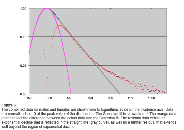
At larger reaction times, another distribution dominates in Figure 6. This is the domain of the reaction time outliers. On this plot, it can be readily discriminated from the exponential decay portion of the curve. Beyond about 820msec reaction time, an event is much more likely to be an outlier than a ‘typical’ reaction event appearing in the exponential tail. This type of analysis is therefore capable of yielding a threshold beyond which we can treat all events as outliers. We have sufficient data to accomplish that discrimination for all age groups.
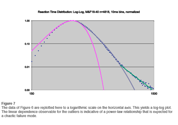
If the data of Figure 6 are re-plotted to a logarithmic scale on the horizontal axis, yielding a log-log plot just as we did in the first newsletter, the outlier distribution is linear, indicating a power-law relationship. This is shown in Figure 7. The data are even more persuasive than before in showing that the outliers are subject to a chaotic failure mode.
It turns out that power laws are ubiquitous in nature—-now that we know to look for them. It is not unlikely that power-law behavior is to be found in the long tail of what appears to be Gaussian-distributed phenomenology, just as was the case here (as well as for EEG band amplitude distributions). But even when the relationship was well established in our awareness, as for example in the case of 1/f-noise in electronic systems and elsewhere, there had been no good model to explain it. That has only occurred over the last couple of decades.
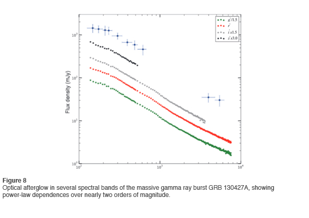
An excellent example of power-law relationships in the current literature is found for the afterglow of a recently observed massive gamma burst. This is shown in Figure 8 for several spectral bands. As is often the case, the governing scaling parameter is not invariant over the whole range. Nevertheless, the power-law relationship clearly represents the best description of the data (Vestrand 2014).
The above description establishes the case that the outliers must be treated as a distinct phenomenon. Further, they must be removed from the further analysis of the main body of the distribution, the ex-Gaussian. Otherwise the analysis of the exponential decay constant (typically called tau) would be severely compromised. This problem is well-known. Outliers are the bane of analysis of Gaussian distributions, and the same goes for the exponential portion. In practice, there is never enough data in a single data set to define the boundary between the exponential decay portion and the outliers. For that purpose, we need the large numbers that the QIKtest database affords us.
Now that the chaotic nature of the outlier phenomenon is well-established, it is worth taking a look at omission errors in that same perspective. After all, there is an obvious kinship between reaction time outliers and omission errors. This will be taken up in the next newsletter on the general topic of the reinterpretation of CPT data.
Reference
Vestrand W.T., et al. (2014). The Bright Optical Flash and Afterglow from the Gamma-Ray Burst GRB 130427A. Science, 343, 38. DOI: 10.1126/science. 1242316